A plain-language companion to the Medusa technical papers

Why does the universe have laws at all? Not why the gravitational constant has a particular value, or why spacetime has four dimensions. The deeper question: why is there any stable mathematical structure to be discovered? Why does an apple fall the same way twice?

One answer is that the universe is built that way. Laws are features of reality, and physics is the process of finding them.

This paper proposes a different answer, motivated by experiment: laws are what any sufficiently constrained observer must build internally in order to predict what happens next. The structure of the law is not a property of the universe alone. It is a property of the relationship between the observer and the universe, specifically, of the constraints under which observation happens.

Paper 1Persistence Structure of Bandwidth-Limited Observation Paper 2Field Equations from Bandwidth-Limited Observation

The observer

A recurrent neural network is placed in a dark room with six sensors arranged in a circle. Somewhere outside the circle, a source emits a signal through a gravitational field. The network receives noisy bursts one after another. It can’t see the source, doesn’t know where it is, and has no concept of gravity, mass, or field equations. Its only job is to predict what the signal will look like at a new location.

The constraints that define it:

Bandwidth-limited: short chunks, not the full continuous signal
Partially observable: only detector signals, never the source directly
Noisy: every measurement has noise
Persistent: it remembers previous episodes and uses that memory

These are the same constraints every human observer faces. We see photons, not atoms. We detect pressure waves, not vibrating strings. We observe in finite windows. We remember.

1. Newton’s law of gravity emerges from prediction

In a weak gravitational field, the observer’s internal representation encodes a potential Φ(r) ∝ 1/r, the exact functional form of Newton’s gravitational law. Shape correlation: 1.000 across all eight seeds. Null controls (no gravity, shuffled detectors) are dead. The observer found 1/r because 1/r is what’s needed to predict accurately.

2. Mass is invisible without change

The observer discovers the shape of gravity immediately. But it cannot distinguish heavy from light. Nine different modifications to the architecture were tested. All failed. Mass remained invisible.

This turns out to be a mathematical theorem, not a bug. The network’s normalization layer strips magnitude from representations, preserving only direction. For a 1/r potential, every derivative scales linearly with mass. After normalization, all masses look the same.

The fix: let the source turn on mid-observation. When the gravitational field appears, the signals at each detector change, and when they change depends on the mass. Heavier sources produce faster changes. The persistent observer detects this temporal pattern. A memoryless observer cannot.

Horizontal bar chart showing seven static architecture interventions all hitting a conformal wall near α_CV ≈ 0.66, while three temporal-quench seeds break through to α_CV ≈ 0.10 — Seven architectural modifications fail to break the conformal wall. Only a temporal quench — letting the field turn on mid-observation — enables mass discrimination.

Every mass measurement in the history of physics works the same way. Archimedes watched water displace. Cavendish watched a torsion bar oscillate. LIGO watches a binary spiral. Kepler watched a planet orbit. Nobody has ever measured mass at rest. The observer independently discovered this principle.

3. Einstein’s field equation from signal transformation

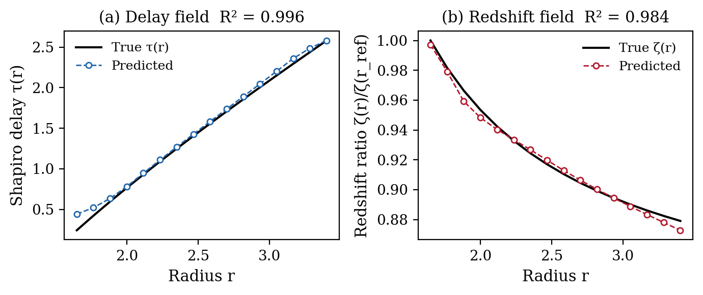
In full Schwarzschild spacetime, signals at different locations differ in two ways: they arrive at different times (delay) and they are stretched to different frequencies (redshift). Both effects depend on the mass, but they are entangled with the source signal itself.

The breakthrough was changing what the observer predicts. Instead of predicting the full signal at each location (512 numbers, mostly about the source), it predicts how the signal transforms between two locations (2 numbers, entirely about gravity). The source waveform cancels. What remains is pure geometry.

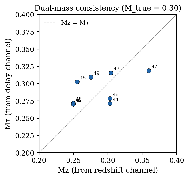
The observer recovers both the delay field and the redshift field. When you fit a mass to each independently, one from how signals stretch, one from how they’re delayed, the two masses agree. That agreement is the Schwarzschild vacuum field equation. The observer was never told about Einstein. It found the relationship because the relationship is what makes predictions accurate.

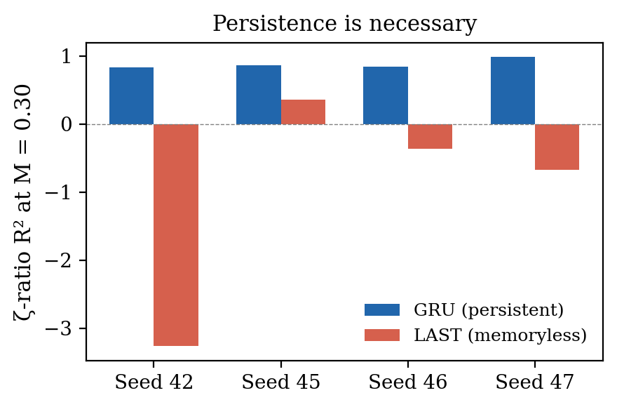
Two panels showing predicted vs true gravitational fields: Shapiro delay τ(r) with R² = 0.996 and redshift ratio ζ(r) with R² = 0.984 — The observer recovers both the delay field (left, R² = 0.996) and the redshift field (right, R² = 0.984) from signal prediction alone.

Scatter plot of mass inferred from redshift vs mass inferred from delay, clustered along the identity line around M = 0.30 — Mass inferred from the redshift channel agrees with mass inferred from the delay channel across eight independent seeds. This agreement is the Schwarzschild vacuum field equation.

4. Persistence is necessary

A memoryless version of the same observer (same architecture, same data, same loss function, just no memory) fails completely on the redshift field. R² = −0.986, worse than guessing the mean. The persistent observer: R² = +0.880.

Bar chart comparing GRU (persistent) R² values near +0.85 against LAST (memoryless) R² values mostly below zero across four seeds — Persistent observers recover the redshift field; memoryless observers fail catastrophically.

Some physical quantities can only be known through persistence, through remembering and comparing across time. A universe of pure snapshots, with no temporal connection between observations, would have geometry but no scale.

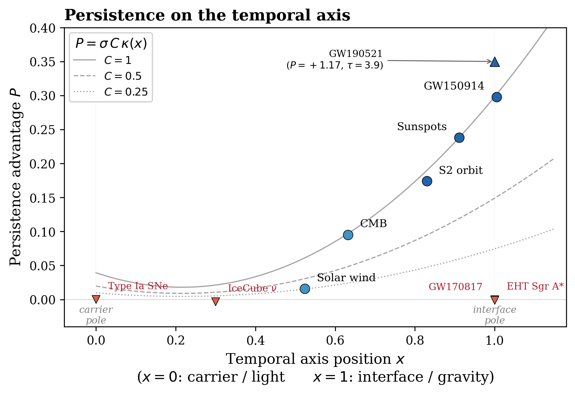
5. The observation manifold

When the same persistent observer is applied to thirteen different physical domains (gravitational waves, radio pulsars, solar magnetograms, stock markets, EEG recordings), the resulting space of observer states forms a manifold organized by a single dominant axis.

At one end: electromagnetic domains where signals are self-explanatory. At the other: gravitational wave interfaces where signals require extended temporal accumulation. The amount of accumulation needed follows a five-parameter law that is architecture-independent: four different neural network architectures produce the same ordering.

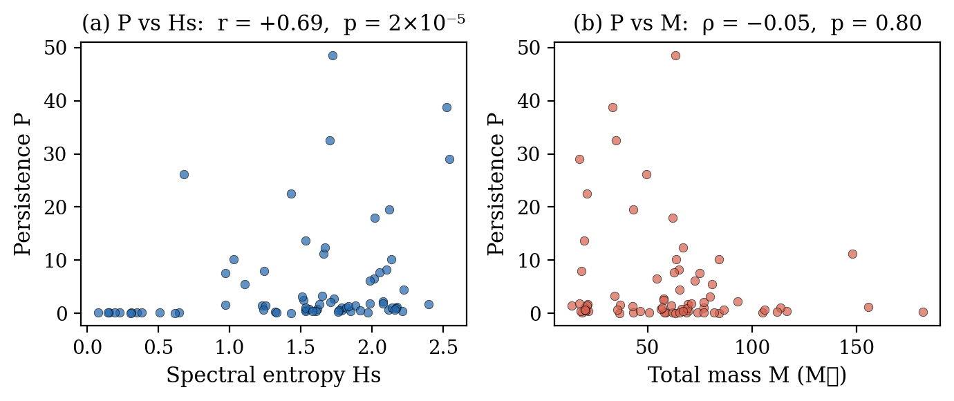
Persistence advantage P plotted against temporal axis position x, showing domains from carrier/light at x=0 to interface/gravity at x=1, with three theoretical κ(x) curves at C=1, 0.5, and 0.25 — Domains placed on the temporal axis. Electromagnetic sources cluster near the carrier pole (x = 0); gravitational wave events cluster near the interface pole (x = 1). The curves show the predicted persistence law P = σCκ(x).

Across 30 binary black hole events from the LIGO/Virgo catalog, persistence correlates with spectral entropy (r = +0.69, p = 2 × 10⁻⁵) and not with mass (ρ = −0.05, p = 0.80). Two systems at identical mass can differ by 100× in how much observation is needed to resolve them. The cost of knowing is not set by what you’re looking at. It’s set by the bandwidth of looking.

Two scatter plots: persistence vs spectral entropy showing strong correlation (r = +0.69), and persistence vs total mass showing no correlation (ρ = −0.05) — Persistence tracks spectral entropy (left, r = +0.69), not mass (right, ρ = −0.05). The cost of observation is set by bandwidth, not by what you’re observing.

What this might mean

If different observers with different architectures converge to the same internal representation, and that representation encodes the field equations, then the law is not a feature of the architecture. It is a feature of the observation problem. The constraints (finite bandwidth, partial observability, noise, persistence) leave very few internal models that support accurate prediction. The field equations may be the unique optimal compression of reality under these constraints.

On the equivalence principle. The persistence law is linear in its depth parameter. If the persistence gradient is interpreted as acceleration, then that acceleration depends on the source but not on the observer. All observers measuring the same source through the same bandwidth experience the same gradient. The equivalence principle, in this framework, is not an assumption. It is a structural consequence.

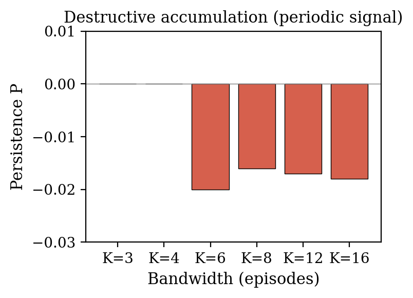
On wave-particle duality. A periodic signal observed through the same pipeline produces no positive persistence when the observer’s episode boundaries do not divide the signal’s period. Accumulating phase-shifted fragments destroys the coherent structure. The observer is better off not accumulating, not measuring which path. This is structurally identical to wave-particle duality: which-path information destroys interference.

Bar chart showing persistence at zero or negative values across all bandwidth settings K=3 through K=16 for a periodic signal — A periodic signal produces zero or negative persistence at every bandwidth. Accumulating phase-shifted fragments is worse than not accumulating at all.

On gravity and quantum mechanics. The observation manifold does not distinguish between gravity and quantum mechanics as separate theories. Gravity appears as the spatial cost of resolving structure. The coherence threshold appears as the temporal cost. Both are consequences of finite-bandwidth observation. If gravity belongs under “measurement constraints” rather than “forces,” then the reason gravity and quantum mechanics have resisted unification may be a categorization error. You do not unify a force with a measurement theory. You notice they were never separate.

What would kill this

A different observer architecture, under the same constraints, converging to a different law.
A memoryless observer recovering the redshift field.
Mass becoming visible in a static conformal field.
Persistence correlating with mass rather than spectral entropy across GWTC events.

None of these has occurred across the tested domains. Four architectures converge to the same structure.

What is established vs. what is proposed

Established by experiment:

Persistent observer recovers Newton’s field equation from signal prediction alone (shape 1.000, 8/8 seeds)
Same observer recovers Schwarzschild redshift (R² up to 0.989) and delay (R² > 0.94) via warp prediction
Persistence is necessary (GRU R² = +0.880 vs memoryless R² = −0.986)
Mass is invisible in static conformal fields and requires temporal symmetry breaking
Observation cost tracks spectral entropy, not mass (r = +0.69 vs ρ = −0.05, 30 GWTC events)
The persistence law is architecture-independent

Proposed as interpretation:

Physical law is the unique optimal compression of reality under observation constraints
The equivalence principle is a structural consequence of linearity in the persistence law
Wave–particle duality is a bandwidth constraint, not a quantum mystery
Gravity and quantum mechanics may be two faces of the same information-theoretic limit

The experimental results stand regardless of whether the interpretations hold.

FAQ

Isn’t this just curve fitting?

The observer was never told what curve to fit. It was trained to predict signals. The 1/r potential, the redshift field, and the delay field all emerged as internal representations because they’re the optimal compression for accurate prediction. Four different architectures converge to the same structure. If it were curve fitting, different architectures would find different curves.

Does this mean the universe isn’t real?

No. The claim is that laws are properties of the observation relationship, the interface between an embedded observer and the world, not that reality doesn’t exist. The universe provides the structure that makes some internal models work and others fail. The observer converges to the field equations because the field equations are what’s actually out there. The point is that the form of the law is constrained by observation as much as by reality.

Why simulated data?

The Newtonian and Schwarzschild results use simulated gravitational fields because you need ground truth to verify the observer recovered the correct potential. You can’t check if a network learned 1/r without knowing the true field. The observation manifold results (Paper 1) use real data from 13 independent instruments: LIGO strain, EHT visibilities, CMB spectra, solar magnetograms, and others. Real-data pipelines for LIGO warp recovery, GPS satellite clock dilation, and NANOGrav pulsar timing are actively under development.

How is this different from just training a neural network on physics data?

Most ML-for-physics work trains a network to solve a known equation or fit a known model. Here the network has no physics in its loss function. It predicts signals. The physics emerges in its internal state because physics is what makes signal prediction work. The critical evidence is architecture independence: GRU, LSTM, ViT, and full-attention Transformer all converge to the same representation. The law is in the problem, not the network.

What does “bandwidth-limited” mean here?

The observer sees short episodes, fixed-length chunks of signal, not the full continuous stream. Like looking through a keyhole at a scene that evolves over time. The bandwidth is the size of that keyhole. When you widen it, the axis positions shift: every domain moves toward “self-explanatory.” There is no absolute frame. The observation cost is always relative to the observer’s bandwidth.

Is this a theory of quantum gravity?

No. The gravitational results are experimentally established. The quantum connection, that accumulation of phase-shifted observations destroys coherent structure, structurally matching wave-particle duality, is an analogy supported by structural correspondence. The paper is explicit that this remains a hypothesis, not a derivation. Whether it extends to a quantitative theory is open.

What’s a “persistence advantage”?

The difference in prediction accuracy between an observer with memory (one that remembers previous episodes) and an identical observer without memory (one that sees only the current episode). Positive means memory helps. Zero means each observation is already complete. The entire framework measures this single number across domains and asks what it depends on.

Has this been peer reviewed?

The papers are preprints on Zenodo. The results are reproducible: all data sources are public, the experimental pipeline is fixed across all domains, and the key findings replicate across four independent architectures and multiple random seeds.

Why Physics Has Laws